Xiaowen Ying

1. Introduction

(This is one of the class project when I was taking the Udacity Self-driving Nano-degree course)

In this project, we are going to design an algorithm to find locate the lane that we are driving. Here is the example of our output.

2. Algorithm Overview

In abstraction, our algorithm follows the following steps to produce the results:

• Compute the camera calibration matrix and distortion coefficients given a set of chessboard images.
• Apply a distortion correction to raw images.
• Use color transforms, gradients, etc., to create a thresholded binary image.
• Apply a perspective transform to rectify binary image (“birds-eye view”).
• Detect lane pixels and fit to find the lane boundary.
• Determine the curvature of the lane and vehicle position with respect to center.
• Warp the detected lane boundaries back onto the original image.
• Output visual display of the lane boundaries and numerical estimation of lane curvature and vehicle position.

3. Camera Calibration

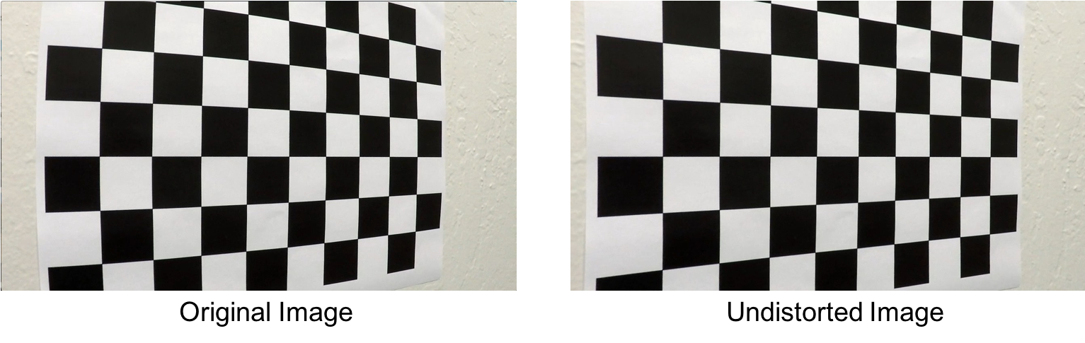
Before we use our algorithm to process the image, we need to calibrate the camera distortion first. In this step, we will load in all the chessboard images and use them for camera calibration. The results will be saved to a file calibration.p for future use.

We start by preparing “object points”, which will be the (x, y, z) coordinates of the chessboard corners in the world. Here we am assuming the chessboard is fixed on the (x, y) plane at z=0, such that the object points are the same for each calibration image. Thus, objp is just a replicated array of coordinates, and objpoints will be appended with a copy of it every time we successfully detect all chessboard corners in a test image. imgpoints will be appended with the (x, y) pixel position of each of the corners in the image plane with each successful chessboard detection.

We then use the output objpoints and imgpoints to compute the camera calibration and distortion coefficients using the cv2.calibrateCamera() function. We apply this distortion correction to the test image using the cv2.undistort() function and obtian this result:

1
2
3
4
5
6
7
8
9
10
11
12
13
14
15
16
17
18
19
20
21
22
23
24
25
26
27
28
29
30
31
32
33
34
35
36
37
38
39
40
41
42
43
44
45
import numpy as np
import cv2
import glob
import pickle

calib_images = glob.glob('camera_cal/*.jpg')

objpoints = [] # 3d points in real world space
imgpoints = [] # 2d points in image plane.

# prepare the object points
objp = np.zeros((6*9,3), np.float32)
objp[:,:2] = np.mgrid[0:9,0:6].T.reshape(-1,2)
# print(objp)

for img_path in calib_images:
	img = cv2.imread(img_path)
	gray = cv2.cvtColor(img,cv2.COLOR_BGR2GRAY)
	ret, corners = cv2.findChessboardCorners(gray, (9,6), None)

	# If the chessboard corners were detected, add them to the list
	if ret == True:
		objpoints.append(objp)
		imgpoints.append(corners)

# Do camera calibration
ret, mtx, dist, rvecs, tvecs = cv2.calibrateCamera(objpoints, imgpoints, gray.shape[::-1], None, None)
calib_config = {}
calib_config['mtx'] = mtx
calib_config['dist'] = dist

pickle.dump(calib_config, open("calibration.p", 'wb'))

# Visualize an example result
test_img1 = cv2.imread(calib_images[0])
undist1 = cv2.undistort(test_img1, mtx, dist, None, mtx)

test_img2 = cv2.imread('test_images/straight_lines1.jpg')
undist2 = cv2.undistort(test_img2, mtx, dist, None, mtx)

cv2.imwrite('output_images/calibrateCamera_original1.jpg', test_img1)
cv2.imwrite('output_images/calibrateCamera_undist1.jpg', undist1)

cv2.imwrite('output_images/calibrateCamera_original2.jpg', test_img2)
cv2.imwrite('output_images/calibrateCamera_undist2.jpg', undist2)

4. Pipeline (single images)

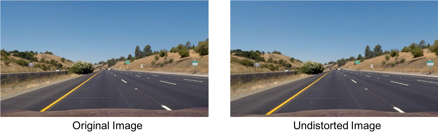
4.1 Correcting Camera Distortion

The process to undistort an image is the same as described in the last part. Here are examples showing the original image and corrected image.

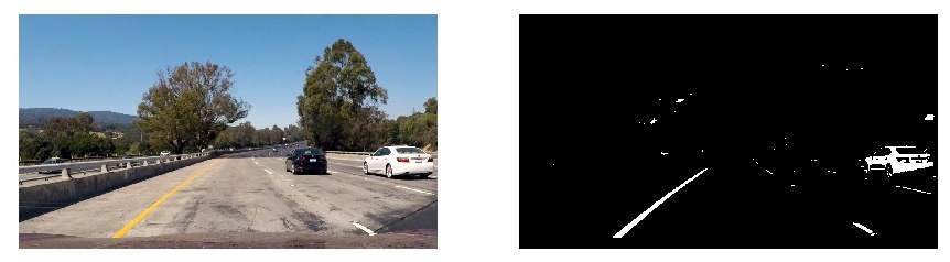
4.2 Creating The Thresholded Image

At the very beginning, I used a combination of color and gradient thresholds to generate the binary image. However, I found this combination is not very robust to deal with yellow lines (sometimes it fails).

During the experiments I have tested different combination of techniques including directional gradient thresholds and different color space select (RGB, HSV, LAB). Finally, I choose to follow some suggestion in a discussion forum to use a combination of L channel in HSL color space and B channel in LAB color space. The B channel in LAB color space works very well on yellow lines but it usually ignores the white lines. L channel in HSL color space is not that strong as the S channel in detecting all the lanes, but it focus more on white colors. Thus the combination of these two color selection works pretty well in my case. Below shows the result after thresholding the image.

4.3 Perspective Transform

Now we need to transform this binary image to a bird-eye view. We create a function called unwarp(). The unwarp() function takes as inputs an image (img), as well as source (src) and destination (dst) points. These points were manually defined.

1
2
3
4
5
def unwarp(img, src, dst):
	M = cv2.getPerspectiveTransform(src, dst)
	Minv = cv2.getPerspectiveTransform(dst, src)
	warped = cv2.warpPerspective(img, M, (img.shape[1], img.shape[0]), flags=cv2.INTER_LINEAR)
	return warped, M, Minv

I verified that my perspective transform was working as expected by drawing the src and dst points onto a test image and its warped counterpart to verify that the lines appear parallel in the warped image. The example will be included in the examples.

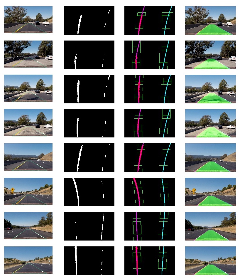
4.4 Examples of intermediate outputs

The figure below shows some examples of outputs at different stages of our algorithm:

5. Pipeline (video)

While running the pipeline on video file, we are not going to detect the lanes from scratch in each frame. Instead, we are holding a Line class that maintains the history and current detection of left and right lanes. If the lanes were detected in the previous frame, we will find the new lanes in the current frame around the previous position. The final lanes for drawing is the average of 5 history fits. This design can generate a more smooth result.